There are a lot of very good resources available on the Internet to learn all about GPS signals, such as ESA Navipedia as well as the actual Navstar GPS interface control documents. This post is mostly a reference for myself about the things I've learned, which might be useful for other people as well.
Radios in general
Before we can talk about GPS specifically, we need to look at radio reception and sampling a bit. So, say we have a signal s(t) occurring around frequency f.
A(t) is the information, which is transmitted. It is much lower in frequency than f, and we can consider it a constant in the time scale of f.
Most radio receivers use a techique called heterodyne as their operating principle. This trick allows the receiver to reduce the frequency of received transmission through the use of a high frequency local oscillator signal. Consider the radio receiver generates two local oscillator signals at frequency f_0, which have a 90 degree phase shift. Let's denote these as


These are both mixed with the received signal in separate mixers, to obtain


To simplify the math, we can think of r_I(t) and r_Q(t) as being the real and imaginary components of a complex signal r(t) as

It also useful to write s(t) in terms of the exponential function as

Since s(t) is real, we can write the mixer outputs as


This allows us to think of m_I(t) and m_Q(t) also as the real and imaginary components of a complex signal m(t)

Consider that f_0 is selected to be close to f. So what we're left with after the mixing is f-f_0, which is a low frequency, and f+f_0, which is a high frequency. We're ultimately not interested in f+f_0, and it just occurs as a side product of the mixing. Since f+f_0 is much higher in frequency than f-f_0, it is straightforward to filter out, and were left with just the low frequency complex signal n(t), which is

A GPS receiver will digitize these signals (the signals denoted as the real part and imaginary part separately) and provide the samples for digital signal processing. It remains particularly useful to consider the signal as complex valued in the DSP. In the digital domain, we can apply the heterodyne concept again, to move the signal to 0 Hz. This allows us to correct for effects caused by Doppler shift for instance.
All this boils down to is taking the actual information A(t) from a high frequency carrier down to very close to 0 Hz. Ideally, we'd like to get A(t) exactly, but without exact timing knowledge, the best we can do is to get A(t) exp(j phi), where phi is some phase error. The information contained in A(t) must be designed in a way, which allows recovering the phase, or it needs to such that the phase error doesn't matter.
GPS signals
With that out of the way, then what and how are the GPS satellites actually transmitting? Well, it turns out that every GPS satellite transmits on the same frequency at the same time. Each of them is basically yelling out their name all the time. Although this results in a cacophony of signals at the receiver side, that name is the key to telling them apart.The name is actually a pseudo random number (PRN) sequence, or PRN code. Each sequence is 1023 bits long, and is transmitted at a 1.023 MHz bit rate, thus repeating every millisecond. The satellites are synchronized so that bit 0 of their respective PRN codes occurs at the same time. If you observe the code of two satellites to not be synchronized to each other, you know that the time it took for the signal to arrive to you from each satellite must be different. This also tells you something (though not everything) about how much farther away one satellite is compared to the other.
The PRN codes above are related to the so-called C/A code transmitted on 1575.42 MHz with BPSK modulation. There are other codes and other frequencies used also in GPS, let alone other GNSS, but I'm not interested in those at the moment. In the following, we'll just happily ignore the other codes, bands and systems.
BPSK modulation simply means, that for each bit in the transmitted bit stream, the A(t) of the transmission has a value of either -1 or 1. For instance A(t)=-1 when the bit transmitted at time t is a 0 and A(t)=1 when the transmitted bit is a 1. The sign will be ambiguous in the reception anyway, so the choice doesn't make a difference.
| PRN codes 1 through 32 encoded as a 1023x32 sized image. Unsurprisingly they mostly look like random noise. |
The PRN sequences have a strong autocorrelation at 0 lag, while having a very weak autocorrelation at any other lag. In addition, the PRN sequence of one satellite has a very weak cross-correlation to the PRN sequence of any other satellite at any lag. In other words, the PRN sequences have a kind of near-orthogonality with everything else but a coherent version of themselves.
It is also useful to consider the PRN code as a sequence of -1 and 1, instead of 0 and 1. This choice results in the strong correlation having a value of 1023, and the weak correlations being close to 0.
 |
| Autocorrelation of PRN code 20. Correlation has a very strong peak at 0 lag, while it is almost 0 elsewhere. Autocorrelations of other PRN codes look similar. |
 |
| Cross correlation between PRN codes 20 and 21. Correlation is almost 0 everywhere. |
It is this near-orthogonality that allows the receiver to separate all the incoming signals from one another. Also, since the correlation exists only at a very precise lag, finding the signal also results in knowing the code phase, which itself is dependent on the time it took for the signal to reach the receiver.
Satellite acquisition
A GPS receiver generates locally the PRN sequence of the satellite it wants to receive, and computes the correlation between the received signal and the generated sequence. If there is a strong correlation, then it knows that it is receiving a satellite with that particular PRN sequence, and that the generated PRN sequence is coherent with the received signal. If there is a weak correlation, then either the satellite isn't visible, or our PRN isn't coherent with the satellite. When searching for a particular satellite, the GPS receiver needs to actually scan through different lags to hopefully find a strong correlation.Unfortunately there is also a second parameter, which the GPS receiver needs to take into account, when finding a satellite. This is the Doppler shift of the received signal (as well as receiver clock frequency error). Although each satellite is transmitting on very precisely 1575.42 MHz in orbit, the motion of the satellite relative to the receiver causes up to 5 kHz difference on the frequency received on ground. Down-conversion without taking the signal Doppler shift into account leaves the receiver with the signal

That is, the phase of the information in A(t) rotates with frequency f_Doppler. In order to properly compute the correlation between the receiver generated PRN and the received signal, this frequency error needs to be quite small. As example, say the correlation integration time is 10 milliseconds, which is pretty typical. If the frequency is off by just 100 Hz, then the phase error makes one complete revolution during the integration time. This results in the latter half of the integration cancelling the result of the first half, and thus will produce a low correlation even if the correlation would otherwise be high. Shorter integration times suffer less from frequency error, but on the other hand suffer more from noise. The receiver thus needs to scan over both the PRN code lags and the Doppler shifts, when searching for a satellite.
Note that the Doppler shift (and receiver clock error) also causes an error in the bit rate seen in the received signal. This could become an issue with very long integration times. This, however, is not a big problem, as the integration time would need to be around 150 milliseconds for half a bit of accumulated error with the maximum expected Doppler shift. In practice, the integration time is limited to 20 ms due to the navigation message bit rate (more on this later).
MAX2769 based receiver
 |
| Data collection setup. Bus Pirate for SPI communication, logic analyzer for data recording. Blue coax leads to a GPS antenna with integrated amplifier. Notice bodge through hole inductor providing bias to active antenna near the antenna SMA connector. |
Now that I understood much more about the GPS signals, I needed to acquire some. There are resources online from which you can get pre-recorded GPS signals to play around with, but where's the fun in that? (Though in all fairness, I did download some samples to play around with before attempting reception of my own).
I set to receive the satellites with a MAX2769 evaluation board, which was donated to me some time ago (thank you Tero!). The MAX2769 is a complete software defined radio frontend meant for receiving GNSS signals. It has an LNA for amplifying the incoming signal. It has a PLL for producing the local oscillator frequency. It has an IQ mixer and the required intermediate frequency filters. Finally, it has the IQ sampling ADC for sampling that intermediate frequency.
I've had a decent amount of problems using the MAX2769, most of which have to do with configuring the IC properly. Many settings are not properly documented in the freely available documentation. Looking around the internet, I found one previous hobby project using the MAX2769. They wanted to go with a direct conversion, having the IF frequency at 0 Hz. I opted not to do that since the documentation is particularly lacking in that part. It's not really clear how anything behaves near DC. In the end, I mostly ended up ignoring the configuration the other project used, and instead made my own conclusions based on the documentation, default values and some testing with an RF generator and a spectrum analyzer. Nothing is set in stone though, and its more than likely I will still change the settings in the future.
The configuration I ended up using in my first reception test is the following:
Register 0: 0xA2919A3
Register 1: 0x8550888
Register 2: 0xEAFF1DC
Register 3: 0x9CC0008
Register 4: 0x0C00080
Register 5: 0x8000070
Register 6: 0x8000000
Register 7: 0x10061B2
This sets the IF to 4.092 MHz with 2.5 MHz IF bandwidth. It enables IQ sampling with 2 bits for both, and sets output mode for unsigned values and signal levels for CMOS. Sample rate is set to 8.184 MHz. To write the configuration, I used a Bus Pirate connected to the SPI port of the IC.
Note that with these settings my IF occurs at the Nyquist frequency. However due to IQ sampling, I can separate positive frequencies from negative frequencies, and thus I'm not actually losing any data (though I might be actually recording the complex conjugate of what I want to record).
The data rate produced by the MAX2769 is somewhat high, producing 4 bits of data at 8.184 MHz. I decided that a logic analyzer would be the most straightforward way to record the data. I used my 8 channel USB connected logic analyzer for the purpose (one of the ubiquitous Cypress FX2LP based logic analyzers).
With everything set, on 2020/03/18 at 22:15 local time in Espoo, Finland, I recorded about 500 milliseconds of data. I had the antenna placed next to a window facing South-South-East. Using a satellite tracking tool I knew there were 12 GPS satellites above the horizon at that time. However some were close to the horizon, and some were not in view from the window.
If you're interested in my data, you can download the data as CSV or binary. Both of these formats are horribly inefficient in storing the data, but are somewhat convenient to use.
The CSV format is simply I,Q per line. Both I and Q get values 0,1,2 or 3. To decode a pair as a complex value, use the formula n_k = (I_k-1.5) + j (Q_k-1.5). Subtracting 1.5 is to reduce the DC content of the signal.
The binary format is simply a dump of numpy.complex type values. To read it, use
n = numpy.fromfile("data_20200318.bin", dtype=numpy.complex)
The contents are the same as for the CSV file and the described decoding.
If you do use the data in either of the formats, remember that it contains a digitization of the intermediate frequency. You should downconvert the signal from 4.092 MHz down to 0. The Fourier transform of the correctly downconverted signal should show power within an about 2.5 MHz band around 0 Hz and look similar to the figure below.
A thing to note is that IF filter center frequency is not exactly at 4.092 MHz even if that's what it is configured to. There should still be enough width to let the GPS signals pass. Also, I haven't made completely sure that the sign of the frequency axis is correct. This would affect at velocity computations, since Doppler shifts would occur with an incorrect sign. Since this data set is simply too short for such things anyway, I won't worry about it too much.
By their very nature, the correlation peaks are very narrow. This makes it difficult to properly visualize them. Nevertheless, a peak can be seen in the figure below (near phase 200, Doppler 0 Hz). I managed to record signals from a GPS satellite!
Not only that, in fact I managed to receive signals from multiple GPS satellites! Below is the same plot computed for PRN code 27 (near phase 550, Doppler -2 kHz). This satellite was also in a favourable position in the sky.
Below is a zoomed-in view of the PRN10 plot - just to enjoy the correlation peak to the fullest 😃
 |
| Satellites visible in the sky from Espoo, Finland on 2020/03/18 22:15 local time. |
If you're interested in my data, you can download the data as CSV or binary. Both of these formats are horribly inefficient in storing the data, but are somewhat convenient to use.
The CSV format is simply I,Q per line. Both I and Q get values 0,1,2 or 3. To decode a pair as a complex value, use the formula n_k = (I_k-1.5) + j (Q_k-1.5). Subtracting 1.5 is to reduce the DC content of the signal.
The binary format is simply a dump of numpy.complex type values. To read it, use
n = numpy.fromfile("data_20200318.bin", dtype=numpy.complex)
The contents are the same as for the CSV file and the described decoding.
If you do use the data in either of the formats, remember that it contains a digitization of the intermediate frequency. You should downconvert the signal from 4.092 MHz down to 0. The Fourier transform of the correctly downconverted signal should show power within an about 2.5 MHz band around 0 Hz and look similar to the figure below.
 |
| Spectrum of recorded data after digital domain downconverison. |
First look
The satellite transmitting PRN10 happened to be quite high in the sky and in the correct direction to not be blocked by the house. In order to find the signal, we can go through the same process a GPS receiver would do to find the satellite. A typical GPS receiver would look at different Doppler shift and PRN phase parameters successively in time. With the recorder data, however, we can go through the same piece of data over and over again until we find the correct parameters. The following figures are produced by computing the correlation of the PRN code against the first 10 milliseconds of recorded data, while stepping through the Doppler from -5 and 5 kHz with 512 steps and through the PRN phases with 8184 steps. The actual correlation result is a complex number because of the phase error we are not yet correcting. The value shown in the figures is the absolute value of the correlation.By their very nature, the correlation peaks are very narrow. This makes it difficult to properly visualize them. Nevertheless, a peak can be seen in the figure below (near phase 200, Doppler 0 Hz). I managed to record signals from a GPS satellite!
 |
| Results of PRN10 acquisition. Do you see the correlation peak? |
Not only that, in fact I managed to receive signals from multiple GPS satellites! Below is the same plot computed for PRN code 27 (near phase 550, Doppler -2 kHz). This satellite was also in a favourable position in the sky.
 |
| Results of PRN10 acquisition. This peak is a bit more difficult to find. |
Below is a zoomed-in view of the PRN10 plot - just to enjoy the correlation peak to the fullest 😃
 |
| PRN10 peak. Now you definitely see it. It's beautiful! |
Navigation message
The PRN code phase alone isn't enough to determine the pseudoranges to the satellites. The PRN code simply repeats too often. The distance difference between satellites is easily more than one light-millisecond (which is about 300 km). Additional information is still needed to determine the delay between the satellites as a number of full milliseconds.
Of course it should come as no surprise, that such information is available in the GPS signal. Turns out that, in addition to the carrier BPSK modulation with the PRN sequence, the PRN sequence itself is BPSK modulated with a bit stream called the navigation message.
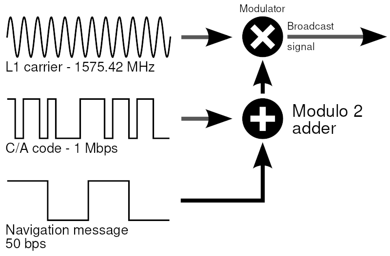 |
| GPS modulation with PRN code and navigation message (figure by P.F. Lammertsma CC BY-SA 3.0) https://en.wikipedia.org/wiki/GPS_signals#/media/File:GPS_signal_modulation_scheme.svg |
Essentially the navigation message will flip the polarity of the PRN code depending on the bit of the navigation message. In other words, the GPS signal A(t) will still be a sequence of -1 and 1 according to the PRN sequence, but which value denotes a 1 and which denotes a 0 gets flipped depending on the navigation message bit.
The navigation message has a bit period of exactly 20 PRN codes, and the bit transitions only occur at PRN code phase 0. Thus the integration periods used for the correlation should always start at code phase 0. I'm not sure if GPS receivers actually do this, but I've used this approach in my implementation.
The navigation message bit stream contains all sorts of useful information that a GPS receiver might needs to know. Such as the aforementioned sychronization data, to allow the proper evaluation of pseudoranges to the satellites. It also contains time information as well as orbit parameters of the satellites. It also includes a short message service type field (GPS Special Message), which I have no idea what it contains. Specification says it can be a short sequence of ASCII characters.
Navigation message in the recorded data
Assume that the Doppler shift is perfectly corrected, the received signal then looks like

Assuming further that A_NAV(t) is constant within each integration period, then correlating this signal against a coherent locally generated PRN code then gives for each integration period i the correlation c_i as

where the amplitude has also been normalized.
These are of course idealized formulas. In reality there is noise on top of the signal also. This noise comes from all typical noise sources, but also from the other satellites since the PRN codes are not perfectly orthogonal.
The correlation thus evaluates as a complex value on the unit circle, and jumps between a point and its antipode as the navigation message bit changes. A GPS receiver will typically constantly adjust for the phase error to align the correlation on the real axis, and thus the value will jump between 1 and -1.
The plots below show what the correlation looks like in time (after meticulous hand-tuning of the Doppler frequency and residual phase error) as well as the effect of using different integration times on the correlation result.


It thus seems obvious that the longest possible integration time is the way to go. Since the navigation message bit period is 20ms, that limits the practical maximum integration time. For best signal to noise ratio, that is the value to use then. Unfortunately it is not possible to know a priori where exactly are the bit transition boundaries of the navigation message. If the 20ms integration period ends up with 10ms of positive polarity and 10ms of negative polarity, then the output is zero.
In the plots above, I've hand-tuned the integration times to occur exactly during the bit periods. The following plots show how the output degrades, if there is an error in synchronizing the bit periods and integration times.


The integration is thus pretty sensitive to the amount of offset. What I understand GPS receiver usually do, is they use a shorter integration time first, and use that to find the bit periods. Then when they know where the transitions occur, they switch to 20ms integration for maximum signal to noise ratio.
For now, the amount of data I have is not enough to do anything useful with the navigation message. There aren't enough bits to determine the time difference between the satellites. For that I'll need to record some more data.
Tracking
The last thing I wanted to cover here is the concept of signal tracking. It is a huge amount of computational effort to go through the data in the way I did. Acquiring the signal does require sweeping over Doppler frequencies and PRN code phases. However, after the signal has been acquired, you don't need to keep looking for it for each successive integration time, since the parameters are quite stable. There are two things to track, the PRN code phase and the signal phase.
Tracking the code phase is typically done by computing the correlations with three phases. These are called the early, prompt and late correlations. The prompt correlation is the best guess of what the PRN code phase is at any given time. The early and late correlations are computed with the code phase being delayed and advanced by a tiny bit (not too much, or we'll lose the correlation completely). If the receiver. for instance, notices that the early correlation is stronger than the prompt correlation, it would adjust the code phase accordingly. This will keep the code phase in lock, as long as it doesn't suddenly change by a large amount.
The code phase drifts because the Doppler shift (and clock errors) cause the PRN bit frequency to look slightly different than 1.023 MHz. As mentioned earlier, at the maximal 5 kHz Doppler shift, this error is half a PRN bit period over 150 milliseconds. The PRN code phase will thus drift by one bit every 300 milliseconds in the most extreme case.
The signal phase error phi needs to be controlled so that it at least stays approximately constant. However, it is useful to control the phase so that the PRN correlation output aligns on the real axis. That is to have phi = 0 or phi = pi. In fact, without the information content in the navigation message, we can't tell them apart.
Given the correlation as
We want to find a correction to signal phase phi, which brings c to the real axis without getting confused about A_NAV changing sign.
The method I used in my tracking experiments was based on the following expression of the phase correction
 ,
,
where it is important to note that we deliberately get rid of quadrant information, hence arctan and not the complex angle.
Thinking about the phase correction as
 ,
,
the arctan correction has two important properties. If c is aligned on the real axis (i.e. when the imaginary component of c is zero) then the correction is also zero.
Second, if c isn't on the real axis, the correction turns c back onto the real axis toward either the positive real direction or negative real direction, depending on which one is closer.
This correction is optimal, in the sense that the corrected phi will turn c exactly to the real axis. On the other hand, it is quite expensive to compute. Due to noise in the signal it is not a good idea to correct for the entire observed error. For stability, the correction should in fact be made as slow as possible. It thus isn't very important if the computed correction is exact or approximate. Approximate corrections can be much faster to compute, and be just as good.
Conclusion
This is about as far as I've managed to get so far in my quest to understand GPS. In addition to Python code for playing around with the recorded data, I've worked on implementing the Doppler shift correction, PRN code generation and integration in Verilog.
It is still some way away from working in practice. However, I can feed the recorded data to the model in Icarus Verilog, and get out the correlation values correctly. However, I haven't yet decided how to output the correlation data from an actual piece of hardware. I think a simple serial line is too slow even for the correlation output.
In addition to IO questions, the Verilog implementation doesn't do any tracking (PRN phase, signal phase) of the signals by itself, and instead needs to be controlled from the outside. In my concept, the FPGA would do only the fast stuff (handling data at 8.184+ Msamples/s), and output a 1 kHz correlation output based on the configuration given to it. This correlation output would be fed to software, which processes it and gives control parameters back to the FPGA to keep the signal locked.
So for this to work in practice, I need to first solve the IO questions, get that data fed to a processor and implement signal tracking software. A soft core might be a viable option, but the FPGA kits I have at hand are quite small.


