Monday, October 2, 2023

Skin and proximity effects

Introduction

In an earlier post I looked at coaxial cables over a ground plane as multiconductor transmission lines. This was to understand quarter wave folded balun operation. Computing the transmission line inductances, however, I realized that the current distribution would depend on how the return current flows.

If the current flows through the center conductor and returns through the shield, the current would be most concentrated on the outside of the center conductor, and return current would concentrate on the inside of the shield. However, if the current flows through the shield and returns through a the ground plane, then the current in the shield would concentrate on the outside part of the shield facing toward the ground plane - and return current would concentrate on the ground plane surface closest to the cable. This concentration of the current is caused by what is known as the skin and proximity effects.

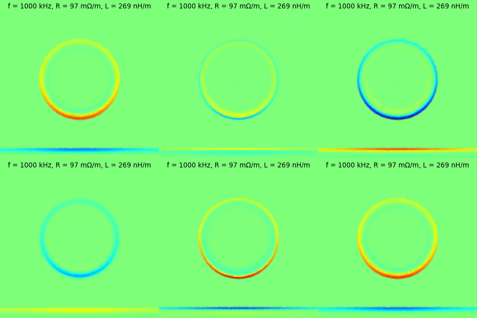
The figures below show a visualization of the current density in a coax under the previously descibed situations. Coax geometry is that of RG316, which is placed very close to a ground plane. The right hand side figure shows the situation where current flows through the inner and back through the shield. while the left hand side shows the situation where current flows through the shield and back through the ground plane. Color indicates current density: dark red is maximal density into the display, dark blue is maximal density out of the display and light green is zero current density. The current is driven by a sinusoidally oscillating uniform electromotive force.


All computations in this article are performed using scikit-fem and my own code, and visualized using matplotlib.

The calculations in my earlier post didn't take these effects into account, and the current assumed a uniform density in the entire conductor in each case. This caused the inductance matrix of the transmission line system to be somewhat incorrect. I mentioned it at the time of writing that post, that accounting for this would be a whole new can of worms. It's now time to open that can.

Deriving the appropriate equations

I'll try to keep the following fairly general, but here we are mostly interested in a long multiconductor transmission line (with n conductors), with dielectrics separating the conductors from each other. The cross-section of the transmission line is assumed to remain constant along its length.

To simplify notation, we'll consider all fields as time-harmonic at frequency w, such that e.g. \(\mathbf{B}(x,y,z,t) = \mathrm{Re} \{ \mathbf{B}(x,y,z) \exp(i \omega t) \}\), and omit the time variable in the following. In particular, we'll omit writing down the time derivative operators and just expand out the result.

Let's start with Ampere-Maxwell's law
\[\nabla \times \mathbf{H} = \mathbf{J} + i\omega \mathbf{D}\]
Inside the conductors we assume Drude's conduction model. The model gives us that \(\mathbf{J} = \sigma \mathbf{E}\) (when considering time scales significantly longer than the mean collision time). Also, it states that there is no polarization in the medium, giving \(\mathbf{D} = \epsilon_0 \mathbf{E}\). (Note: alternatively we could have assumed that there is no conduction current \(\mathbf{J}\), but that we're dealing with an extremely lossy dielectric medium. This would have been represented by a large imaginary component of the permittivity).

Following Drude, inside the conductor we have
\[\nabla \times \mathbf{H} = \sigma \mathbf{E} + i\omega \epsilon_0 \mathbf{E}\]
However, for copper and the frequencies we're intersted in, \(\sigma \mathbf{E}\) dominates \(i\omega \epsilon_0 \mathbf{E}\) by more than a factor of a million, so we'll ignore the term \(i\omega \epsilon_0 \mathbf{E}\).

Inside the insulators we assume no conduction and that \(\mathbf{D} = \epsilon \mathbf{E}\), where \(\epsilon\) is the permittivity of the insulator (and is taken as different within each material). This gives
\[\nabla \times \mathbf{H} = i\omega \epsilon \mathbf{E}\]
Again, for the materials and frequencies we're interested in, \(i\omega \epsilon \mathbf{E}\) significantly smaller than \(\sigma \mathbf{E}\), and thus we can ignore this source of the magnetic field.

For simplicity, let us assume that all magnetic materials are linear and isotropic, and thus that the constitutive relation \(\mathbf{H} = \mu^{-1} \mathbf{B}\) holds within each material, where mu describes the permeability of the material (and is taken as different within each material).

So, thus far, inside the conductors we have
\[\nabla \times (\mu^{-1} \mathbf{B}) = \sigma \mathbf{E}\]
and elsewhere
\[\nabla \times (\mu^{-1} \mathbf{B}) = 0\]
To simultaneously also satisfy Gauss's law for magnetism and Faraday's law, let us take the potential field approach by introducing the magnetic vector potential \(\mathbf{A}\) and the electric potential \(\varphi\), such that \(\mathbf{B} = \nabla \times \mathbf{A}\) and \(\mathbf{E} = -\nabla \varphi - i\omega \mathbf{A}\).

Thus inside the conductors we have
\[\nabla \times (\mu^{-1} \nabla \times \mathbf{A}) = -\sigma \nabla \varphi - i \omega \sigma \mathbf{A}\]
while elsewhere
\[\nabla \times (\mu^{-1} \nabla \times \mathbf{A}) = 0\]

Solving the equations

Take the geometry as such that the transmission line is directed along the \(z\) coordinate direction.  The cross-sectional geometry of the transmission line is then the \(xy\) plane. Consider then that for each conductor \(c\) our electric potential is such that \( (\nabla \varphi)(x,y) = -U_c \mathbf{e}_z\), when \( (x,y) \in \Omega_c\), where \(\Omega_c\) is the cross-section surface of conductor \(c\), and \(U_c\) is a given constant value. In other words, consider that for each conductor \(c\), we have some voltage drop of \(U_c\) per unit length which drives the current in the conductor.

Assume then that \(\mathbf{A} = \mathbf{A}(x,y)\), i.e. that \(\mathbf{A}\) is only a function of position in the cross-section of the transmission line and does not vary in the length-wise direction (i.e. the transmission line is long). It then follows (though not entirely trivially) that \(\mathbf{A}(x,y) = A(x,y) \mathbf{e}_z\), and our problem actually reduces to a two-dimensional scalar problem in the \(xy\) plane.

For such an A, we have
\[\nabla \times (\mu^{-1} \nabla \times \mathbf{A}) = -\nabla \cdot (\mu^{-1} \nabla A) \mathbf{e}_z\]
Thus, inside conductor \(c\) we have the scalar problem
\[i \omega \sigma A - \nabla \cdot (\mu^{-1} \nabla A) = \sigma U_c\]
while outside the conductors
\[-\nabla \cdot (\mu^{-1} \nabla A) = 0\]
With finite elements, and a finite computation domain, we must consider boundary conditions also. We choose to enforce the boundary condition \(\nabla A \cdot \mathbf{n} = 0\), which corresponds with the magnetic field being normal to the boundary. (Note: the boundary condition \(A = 0\) corresponds with the magnetic field being tangential to the boundary). Our choice of boundary condition results in all currents in the system always getting automatically balanced, although it's otherwise a somewhat dubious condition to enforce. The domain must be large enough that these edge effects become negligible.

The problem is then solved using standard finite element methods. The solution of course gives the magnetic vector potential. To find the currents in the conductors, we'll need to do some post-processing still. For this, we'll recall that
\[\mathbf{J} = \nabla \times (\mu^{-1} \mathbf{B}) = \nabla \times (\mu^{-1} \nabla \times \mathbf{A})\]
Let's denote \(\mathbf{J} = J \mathbf{e}_z\), so that for the scalar current density field we have
\[J = -\nabla \cdot (\mu^{-1} \nabla A),\]
which is very straightforward to compute from \(A\) using our finite element approach. Further, the total current in conductor \(c\) is then the integral
\[I_c = \int_{\Omega_c} J\ \mathrm{d}\mathbf{x}, \]
where \(\Omega_c\) is again the cross-section surface of conductor \(c\).

Consider then that the voltage gradient applied across conductor \(c\) was \(U_c\). This allows the conductor currents to be described by the admittance matrix \(\mathbf{Y}\) of the system as
\[\begin{pmatrix} I_1 \\ I_2 \\ \vdots \\ I_n \end{pmatrix} = \mathbf{Y} \begin{pmatrix} U_1 \\ U_2 \\ \vdots \\ U_n \end{pmatrix}\]
or
\[\mathbf{I} = \mathbf{Y} \mathbf{U}\]
To find the admittance matrix of our system, we can solve the currents \(\mathbf{I}\) a total of \(n\) separate times, each time using a different linearly independent set of voltage drops. For example, we can take \(\mathbf{U}\) as each of the members of the canonical basis in turn and solve the currents.

Perhaps an even more useful way to look at the system is the impedance matrix, which is the inverse of the admittance matrix.
\[\mathbf{Z} = \mathbf{Y}^{-1}\]
We expect that our system has some resistance, which is due to the resistivity of the conductors. This would be described by the real part of the impedance matrix. The system is also expected to exhibit inductive reactance, which is described by the imaginary part of the impedance matrix. Dividing the reactance by \(\omega\) gives us the inductance. Thus, the inductance matrix of the system is simply the imaginary part of the impedance matrix divided by \(\omega\)
\[\mathbf{L} = \omega^{-1} \mathrm{Im}\{ \mathbf{Z}\}\]

Applications

Skin effect in a circular conductor

A copper conductor of 1 mm diameter is subjected to various frequencies of AC excitation. The permeability of both copper and air in this system are taken as approximately \(\mu_0\), which is the vacuum permeability.

Current density is visualized in the cross-section surface with color, but also along the diameter as a 1D plot.

Coaxial cable

A coax of RG316 dimensions
  • Inner conductor OD: 0.53 mm
  • Inner insulator OD: 1.53 mm
  • Outer conductor OD: 1.98 mm
  • Outer insulator OD: 2.5 mm
is placed over a ground plane, with center to plane height 1.75 mm. All conductors are made of copper, while \(\mu \approx \mu_0\) for all materials, where \(\mu_0\) is the vacuum permeability.


Consider the two cases:
  1. Current is balanced between inner and outer conductors: no current flows through the ground plane
  2. Current flows through the outer conductor and ground plane: no current flows through the inner conductor

Inner - outer


Outer - ground plane


Differential microstrip

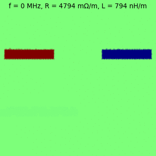
Take a differential microstrip of dimensions
  • Trace width: 0.2mm
  • Trace separation: 0.2mm
  • Trace thickness: 0.035mm
  • PCB layer thickness: 0.2mm
All conductors are made of copper, with \(\sigma = 5.96\ \mathrm{S} \mathrm{m}^{-1}\) while \(\mu \approx \mu_0\) for all materials, where \(\mu_0\) is the vacuum permeability.


Consider two cases:
  1. The current enters the left conductor and returns via the right conductor: the odd mode
  2. The current enters through both the left conductor and the right conductor and returns through the ground plane: the even mode

Odd mode

Even mode


Observations

The higher the frequency, the more concentrated the current and return current are toward each other. With increasing frequency the current is passing through an ever decreasing cross-sectional area. Thus the resistance increases with frequency. On the other hand, the closer the opposite currents are moving to each other, the more the resulting magnetic fields cancel each other out. Thus the inductance decreases with increasing frequency.

Sunday, March 19, 2023

GPS Special Messages

The GPS ICD (specifically Appendix II of the document IS-GPS-200) specifies something called Special Messages transmitted in the GPS LNAV message. The field, which is transmitted as page 17 of subframe 4, is described as "specific contents at the discretion of the Operating Command" and that "it shall accommodate the transmission of 22 eight-bit ASCII characters". As ASCII tends to be used for encoding text, this sounds like a global one-way short message service.

To add to the mystery of this message, there doesn't appear to be any further information about this message online. It is sometimes mentioned as being part of the LNAV message with some quote of the ICD text. I have not been able to find anything on the contents. Is it actually in use? What are the actual data contained within? Given that the LNAV data is globally broadcast, it's surprising that this information is not readily available.

Over a few years, I've been on-and-off learning about GPS by attempting to build my own GPS receiver. This spring I've got the point where I can track a satellite in real-time and collect data from it. On March 15 (around 20:45 UTC). I got several minutes worth of good data from PRN 32. Among the data was one instance of page 17 of subframe 4. I decoded the content of the special message as:

N9Y2L L'O:CJL O2AY"WMG

The parity bits of all words in the subframe were correct, and the decoded characters match the valid character set defined in the ICD. Overall I'm very confident that I have decoded the contents correctly. The field is thus obviously in some use. but it's a bit of a dissapointment that the meaning of the contents is not immediately obvious.

Now, it's not yet clear to me if all satellites transmit the same message. In fact, it's not even clear if a single satellite transmits the same contents on each message repetition. I'll be looking into these in the future as I get more data :-)

Sunday, November 21, 2021

How GPIB really works

In a post long ago I wrote about having built a serial ULI GPIB interface adapter, and about some of the troubles I had with the original firmware of that adapter. I meant to fix those issues in the firmware, but I've come to realize that ULI is never going to properly work over serial, and I'll need to come up with a custom solution and to re-write the firmware.

To do that, I've researched how GPIB actually works. A bit surprisingly, the resources available on the topic are pretty bad. I thought that there'd be several detail resouces on the subject. I even acquired a copy of the original IEEE-488-1978 standard, and while it helped, it is written in (IMHO) a very difficult to understand way. In the end I've tried to piece together the information from several sources and from testing with how my GPIB enabled instruments behave. This post is mainly me documenting my findings to myself for later reference.

Basic behavior

There is at most one talker on the bus at a time, while there can be several listeners. The controller determines which device is the talker and which are listeners at any given time. Almost always the controller is either the talker or a listener on the bus.

Data output by the talker on the bus is read in by all of the listeners. This would allow e.g. a measurement device to produce output as a talker and a data recording device to collect it as a listener. In my use cases, the data would be always between a single instrument and the controller. I would consider it to be very rare these days, that data would get passed directly from one instrument to another.

The controller can act as a talker and as a listener, but in addition it can send commands.

The signals

All signals, including data lines, operate with inverted logic. That is, a high level voltage is a 0 and a low level voltage is a 1. In particular, control lines are asserted when a low voltage level is present and deasserted when a high voltage level is present. The logic level voltages themselves are TTL.

When used as outputs, the signals are driven with one of two driver types. Some signals are open-collector with weak pull-ups, while others are push-pull driven. The data lines use both driver types in different conditions, while for the other lines the driving scheme is fixed. All lines are high-impedance on a device, when they are used as inputs.

Open-collector drive is used to produce a wired OR on the bus for certain lines. In this case the low level (value 1 or asserted state) is the dominant state.

ATN

Attention. Asserted by the controller to signal the sending of a command on the data lines. This line is push-pull driven by the controller and is high-impedance on the other devices.

IFC

Interface clear. Asserted by the controller to asynchronously reset the bus logic in devices. This line is push-pull driven by the controller and is high-impedance on the other devices.

REN

Remote enable. Asserted by the controller to cause addressed devices enter remote operation mode (local user interface disabled, except for go to local key). This line is push-pull driven by the controller and is high-impedance on the other devices.

SRQ

Service request. Asserted by any device requesting an interrupt from the controller. Reason is device dependent. This line is open-collector driven by every other device on the bus except for the controller. It is high-impedance on the controller.

EOI

End or Identify. This signal has two meanings.

End: Can be asserted by a talker to indicate the last byte of a data transfer.  It is push-pull driven by the talker and is high-impedance on the other devices. It appears to be talker implementation specific if it is asserted at all, as well has how it is interpreted by listeners when it is asserted. As an example, my Racal-Dana 1992 does not assert EOI when talking, but does accept EOI as an end-of-line indicator if it is asserted. However, it also accepts CRLF as an end-of-line even without EOI asserted.

Identify: Asserted by the controller to request parallel polled devices to identify if they have a service request. It is push-pull driven by the controller and is high-impedance on the other devices. Parallel poll in general seems to be very rarely used, and is up to the controller to use it anyway. So when programming a controller, the whole functionality can be omitted.

NRFD

Not ready for data. Asserted by any listener on the bus, which is not ready to receive data. This line is open collector driven by all listeners on the bus, while it is high impedance for others. Since the asserted state is dominant, the bus will show NRFD as asserted if any one listener is not ready.

DAV

Data valid. Asserted by the talker to indicate that the data lines contain valid data, which should be accepted by the listeners. The talker waits for the NRFD signal to become deasserted before asserting DAV. This line is push-pull driven be the talker while it is high impedance on other devices.

NDAC

Not data accepted. Asserted by any listener on the bus, which has not yet accepted the valid data on the bus. This line is open collector driven by all listeners on the bus, while it is high impedance for others. Since the asserted state is dominant, the bus will show NDAC as asserted if any one listener has not accepted the data. After all listeners have accepted the data, the talker knows to de-assert the DAV line and prepare the next data.

D1 through D8

Data lines. These contain the data that is being sent. It is important to note that data lines also operate with inverted logic. The lines are push-pull driven by the talker, or open collector driven by polled devices when a parallel poll identify is requested by the controller. For other devices, the lines are high impedance.

Handshaking

At the core of transmitting data and commands is the three-way handshake process. This allows the data to be transmitted asynchronously, and following the limitations of the slowest device involved with the transfer.

Handshake timing

The listeners first deassert their pull of the NRFD line when they become able to receive data. When the last of the listeners releases the line, the line goes high (deasserted). This signals the talker that they can now transmit data. Before beginning the transfer, the talker should check that NRFD and NDAC are not both high, as that would be an indication that there is no-one listening (though at least my Racal-Dana 1992 does not do such checking).

The talker then sets the data on the data lines (remembering that the logic is inverted) and asserts the DAV line to indicate valid data (note: data can be set on the data lines already before NRFD goes high, as long as data is stable when DAV is asserted). There should be a delay of at least 1.5us between setting the data on the data lines and assertion of DAV to ensure the settling of the data lines (required by the standard).

Asserting the DAV line will signal the listeners to receive the data. When a listener has accepted the data, it will again assert the NRFD line (i.e. pull it low) to indicate that they are not ready for new data and will release their pull on the NDAC line. The NRFD line on the bus will thus become again asserted as soon as the first listener has accepted the data, but the NDAC line will become deasserted only after the last listener has accepted the data.

When the NDAC line becomes deasserted, it signals the talker that all listeners have accepted the data, and the talker will deassert the DAV line. After this, when the listeners are again ready to receive more data, they will again release their pull on NRFD line and the cycle begins again.

Exactly the same handshake cycle is used for transmitting commands when the ATN line is asserted. In that case however, the talker is the controller and the listeners are all devices on the bus.

Commands

As said, the commands are sent by the controller on the data lines together with the ATN asserted. Asserting the ATN line will instantly (<200ns) cause the other devices to release the bus for the controller to talk.

The command will be transmitted on the data lines of the bus following the handshaking protocol. The controller acts as the talker, while the other devices will act as listeners. Each command that the controller sends is a single byte.

A large portion of the commands are reserved commanding specific devices to become listeners or talkers. The addressing is also used together with the addressed group of commands, which only affect devices which have been addressed. Each addressable device on the bus has a GPIB address. The GPIB address of a device is a 5 bit value between 0 and 30 (with value 31 reserved for a special purpose).

Some sources say that address 0 is often reserved for the controller itself, but this makes no sense to me. The controller is the only one addressing the other devices, so it has no need for an address. I guess it makes sense in the weird situation, where there are several possible controllers that need to address each other.

Listen - 0x20+GPIB address - MLA

A device will become a listener if it receives the listen command with its address.

In the GPIB nomenclature the value "0x20+GPIB address" is called the listen address of the device, which is a bit misleading since this is actually the full command for the device to begin listening. Upon reception of its listen address, a device will stop being a talker (if it was one) and begin acting as a listener.

To set a device as a listener, the controller does the following

  1. Assert ATN (and set proper bus directions)
  2. Send the value "0x20+GPIB address" (MLA) on the data lines using the handshake protocol
  3. Deassert ATN (and set proper bus directions)

The configured device will handshake data sent on the bus and interpret them in a device dependent way.

Unlisten - 0x3f - UNL

All devices currently listening will stop listening when they receive the unlisten command. The unlisten command is basically the listen command issued for address 31, which is why no device can have GPIB address 31.

Talk - 0x40+GPIB address - MTA

A device will become a talker if it receives the talk command with its address.

In the GPIB nomenclature the value "0x40+GPIB address" is called the talk address of the device. Upon reception of its talk address, a device will stop being a listener (if it was one) and begin acting as a talker. Upon reception of a talk address of any other device it will cease acting as a talker (if it was one).

To set a device as a talker, the controller does the following

  1. Assert ATN (and set proper bus directions)
  2. Send the value "0x40+GPIB address" (MTA) on the data lines using the handshake protocol
  3. Deassert ATN (and set proper bus directions)

Untalk - 0x5f - UNT

The current talker will stop talking when it receives the untalk command. The untalk command is essentially just the talk command issued for address 31.

Interface clear

Asynchronously reset the GPIB interfaces of the devices on the bus. To perform the clear, the controller asserts the IFC control line for more than 150 microseconds. Devices forget their listen/talk status etc. Measurement etc. states of the instruments may be retained.

Remote control

Enabling remote control of devices uses its own REN control line. As long as the REN line is asserted, the devices which have been put into remote control stay in remote control. When the REN line is deasserted, then all devices go back to local control asynchronously.

To set a specific device to remote control, the controller does the following

  1. Assert ATN (and set proper bus directions)
  2. Assert REN
  3. Send the value "0x20+GPIB address" (MLA) on the data lines using the handshake protocol
  4. Deassert ATN (and set proper bus directions)

Any device addressed to listen while the REN message is asserted goes into remote control. The addressed devices will remain listeners. The controller can send the UNL command if the devices shouldn't be a listeners at this time. The device will remain in remote mode for as long as REN is asserted or a go to local command is issued (either via manual entry from keypad or through command).

Local lock out - 0x11 - LLO

Will cause the go to local (or equivalent) button to be disabled on the from front panels of all instruments. This command does not inherently take devices to remote control, and doesn't an effect if the device is not taken to remot control.

To cause a specific device to enter remote control with local lockout, the controller does the following

  1. Assert ATN (and set proper bus directions)
  2. Assert REN
  3. Send the value 0x11 (LLO) on the data lines using the handshake protocol
  4. Send the value "0x20+GPIB address" (MLA) on the data lines using the handshake protocol
  5. Deassert ATN (and set proper bus directions)

After the LLO command has been issued with REN asserted, any following listen command will place a device into remote control with go to local disabled. The controller can send the UNL command if the device doesn't need to be a listener at this time. The device will remain in remote control as long as REN is asserted or a go to local command is issued. As long as REN is asserted, any device transitioning to remote control will have their go to local disabled. To re-enable the go to local buttons, REN needs to be deasserted.

Go to local - 0x01 - GTL

Will cause the addressed devices to go back to local control even when REN is asserted.

To send the GTL command to a specific device, the controller does the following

  1. Assert ATN (and set proper bus directions)
  2. Send the value 0x3f (UNL) on the data lines using the handshake protocol
  3. Send the value "0x20+GPIB address" (MLA) on the data lines using the handshake protocol
  4. Send the value 0x14 on the data lines using the handshake protocol
  5. Deassert ATN (and set proper bus directions)

Device clear - 0x14 - DCL

Will cause a power-on-reset type resetting of device functions for all devices on the bus. Racal-Dana 1992 will only perform this reset if it is under remote control, but I'm unclear if this is common (IEEE-488-1978 specifies this without remote). In any case, the devices at least don't need to be addressed to follow the command.

To clear devices on the bus, the controller does the following

  1. Assert ATN (and set proper bus directions)
  2. Send the value 0x14 (DCL) on the data lines using the handshake protocol
  3. Deassert ATN (and set proper bus directions)

Selected device clear - 0x04 - SDC

Will cause a power-on-reset type resetting of device functions for the devices addressed to listen on the bus.

To clear a specific device on the bus, the controller does the following

  1. Assert ATN (and set proper bus directions)
  2. Send the value 0x3f (UNL) on the data lines using the handshake protocol
  3. Send the value "0x20+GPIB address" (MLA) on the data lines using the handshake protocol 
  4. Send the value 0x04 (SDC) on the data lines using the handshake protocol
  5. Deassert ATN (and set proper bus directions)

Group execute trigger - 0x08 - GET

Causes a trigger event to be issued to the devices addressed to listen on the bus. What the trigger means is device dependent. On the Racal-Dana 1992 it triggers a single shot measurement.

To issue a trigger to a specific device on the bus, the controller does the following

  1. Assert ATN (and set proper bus directions)
  2. Send the value 0x3f (UNL) on the data lines using the handshake protocol
  3. Send the value "0x20+GPIB address" (MLA) on the data lines using the handshake protocol 
  4. Send the value 0x08 (GET) on the data lines using the handshake protocol
  5. Deassert ATN (and set proper bus directions)

Serial poll enable - 0x18 - SPE

Causes all devices on bus to send status messages instead of data, when commanded to talk.

This is used by the controller to determine which device asserted the SRQ line. The other mechanism for determining this is the parallel poll, but it seems rather obscure and rarely worth the effort.

To find the devices, which asserted the SRQ, the controller does the following

  1. Assert ATN (and set proper bus direction)
  2. Send the value 0x3f (UNL) on the data lines using the handshake protocol
  3. Send the value 0x5f (UNT) on the data lines using the handshake protocol
  4. Send the value 0x18 (SPE) on the data lines using the handshake protocol
To poll whether device with GPIB address X asserted SRQ:
  1. Assert ATN (and set proper bus direction)
  2. Send the value "0x40+X" (MTA) on the data lines using the handshake protocol
  3. Deassert ATN (and set proper bus direction)
  4. As a listener, receive the single byte status message from the talker using the handshake protocol
The status message byte holds the the SRQ status as bit 6. The controller polls each device, until if finds the one that asserted the SRQ. The status byte may also contain other device dependent information.

Serial poll disable - 0x19 - SPD

Causes all devices on bus to again send data instead of status messages, when commanded to talk.

Other commands

Parallel poll configure - 0x05 - PPC (Parallel poll stuff...)
Parallel poll enable - 0x6X - PPE (Parallel poll stuff...)
Parallel poll disable - 0x7X - PPD (Parallel poll stuff...)
Parallel poll unconfigure - 0x15 - PPU (Parallel poll stuff...)
Take control - 0x09 - TCT (Cause another controller to become the controller)

Interface ICs

The common interface ICs used for GPIB communications are the Texas Instruments SN75160B, SN75161B and SN75162B.

The SN75160B is an octal tranceiver, which is commonly used for the data bus signals. It allows setting the data lines into receive or transmit via the talk enable (TE) signal (TE=high, transmitting toward GPIB). When in transmit mode, the bus-side output can be set as either push-pull or open-collector via the pullup enable (PE) signal (PE=high, outputs are push-pull). The datasheet of the IC is annoyingly unclear on these aspects. It is important to note that a high value on one side of the tranceiver is transmitted as high value on the other side. That is, there are no inverters in the interface to account for the inverted logic on GPIB.

The open-collector drive capability of the data lines seems to be used only for the parallel poll feature. For the sole controller on the bus, the data lines are always either push-pull driven toward the bus or used as inputs. That is, PE can be kept constantly high.

The SN75161B and SN75162B are tranceivers for the GPIB control lines. One difference between the two is than the SN75162B includes a separate direction control for ATN/SRQ and REN/IFC, while on the SN75161B there is a single control for all four. They also seem to have different drive circuitry for some of the lines. My interface is built using an SN75162B, so I'll only cover it here.

The direction of the controller lines ATN, SRQ, REN and IFC are controlled via the DC and SC lines.

  • When SC is high, REN and IFC are push-pull outputs toward the bus.
  • When SC is low, REN and IFC are inputs from the bus.
  • When DC is low, ATN is a push-pull output toward the bus and SRQ is an input from the bus.
  • When DC is high, ATN is an input from the bus and SRQ is a open-collector output toward the bus.

For the sole controller on the bus, the SC line can be kept constantly high and the DC line can be kept constantly low.

The direction of the handshake lines NRFD, DAV and NDAC are controlled via the TE line.

  • When TE is high, DAV is a push-pull output toward the bus, while NRFD and NDAC are inputs from the bus.
  • When TE is low, DAV is an input from the bus, while NRFD and NDAC are open-collector outputs toward the bus.
Similar to the SN75160B, there are no inverters inside the SN75162B to account for the inverted logic of the GPIB.